
Welcome to the first installment of Reproducible Finance by way of Alpha Architect. For the uninitiated, this series is a bit different than the other stuff on AA – we’ll focus on writing clean, reproducible code, mostly R (but some python too), applied to different ideas from the world of investing. We won’t delve deep into those ideas because the goal is to get familiar with the code. Let’s kick it off with the good’ol investment strategy called Momentum.
Q2 hedge fund letters, conference, scoops etc
Before we even tiptoe in that direction, please note that this is not intended as investment advice and it’s not intended to be a script that can be implemented for trading. The goal is to explore some R code flows applied to a real-world project. Don’t live trade this at home!
Momentum Research with R
In a previous post, we covered the steps for implementing a basic momentum investing strategy with R code. We covered quite a bit of code in that post and it’s worth a look if momentum investing or algorithmic (fancy word for if/else) logic is new to you (if R code is brand new, a good place to start this post on calculating prices and returns with R). Today, we’re going to tackle a slightly different momentum project and focus on the idea of quality.
Streaming through the literature on momentum investing is the idea that some types of momentum are of higher quality, and therefore more attractive, than others. For example, we can imagine two stocks that trade for 100 dollars on January 1 of year 1. Stock 1 gains about one dollar per month for the next 12 months, for a cumulative gain of 12%. Stock 2 zigzags around, going up two dollars one month, down 4 dollars the next, then finally receives some positive new, pops in January of year 2 and ends at $112. Same cumulative 12-month returns, but very different return profiles. Is one a more attractive candidate for a momentum strategy? Today we’ll look at two methodologies that would classify Stock 1 as the more attractive.
The first methodology comes from Grinblatt and Moskowitz 2004(1) and examines whether during the previous 12 months of returns, 8 out of the 12 months were positive, in addition to whether the past returns meet our momentum criteria from last time. If at least 8 of the past 12 months’ returns were positive, we label that a 1 to indicate a positive measure of quality. That’s just one idea from their paper that we’ll code up today, there’s lots more to explore for the curious!
The second measure of quality is covered on alpha architect here and conceives of an asset’s price history as reflecting either continuous information or discrete information. Continuous information manifests itself as gradual price increases, indicating that perhaps the market isn’t fully reflecting the information that has arrived. Discrete information manifests itself immediately and with near completeness. Imagine an FDA drug approval that sends a price skyrocketing the day it’s announced, indicating that the market is fully reflecting the information. If the positive news is fully priced in, we can’t take advantage of the momentum anomaly.
This Information Discreteness (ID) is captured numerically with the following equation:
ID = sign(PRET) * (% months negative – % months positive)
where PRET is the cumulative return over the preceding 12 months. A negative value for ID indicates continuous information (high-quality momentum). Notice that the smallest possible value of ID is -1 (say, 12 positive months and a positive cumulative return) and the largest possible value is 1 (say, all negative months and a negative cumulative return). If there are mostly positive months and the sign of the cumulative returns is positive, the ID will be near -1, signaling continuous information and quality momentum. Conversely, if most of the returns are negative, but the cumulative return is still positive, it will result in a positive ID, signaling discrete or low-quality momentum. I highly recommend the full paper for more background.
Building Grinblatt and Moskowitz Momentum
Let’s get to the R code, starting with methodology 1, wherein we determine whether at least 8 of the past 12 months showed a positive return. We’re going to do things a bit differently from last time where we examined a momentum strategy that used SPY and EFA. Today, we’ll work with SPY, XLF and XLE and try to compare the quality of their momentum signals. That means we’ll need to calculate their monthly returns and their past 12-months’ returns.
We’ll import daily prices, convert to monthly returns, and then create a new column called skip_mon_return that is the one month lagged returns. We do that because the most recent previous month might be a bit noisy or volatile, and leaves us at the mercy of the so-called short term reversal effect.
Let’s start by loading our packages for today,
library(tidyverse)library(highcharter)library(tibbletime)library(tidyquant)library(timetk)library(riingo)riingo_set_token(“your token here”)
Then we’ll import price data from tiingo, using the R package called riingo.
symbols <- c(“SPY”, “XLF”, “XLE”) prices_daily <-
symbols %>% riingo_prices(., start_date = “2000-01-01”, end_date = “2018-12-31”) %>% mutate(date = ymd(date)) %>% group_by(ticker)
Now let’s convert to monthly prices.
prices_monthly <- prices_daily %>% tq_transmute(select = adjClose,
mutate_fun = to.monthly,
indexAt = “lastof”)
And finally, convert from monthly prices to monthly returns. We’ll also lag our returns and place the lagged values in a new column called ‘skip_mon_return’.
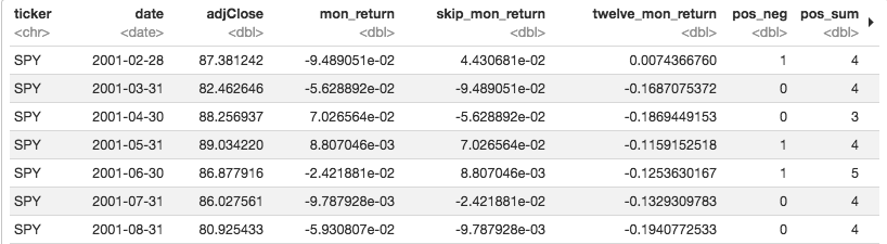
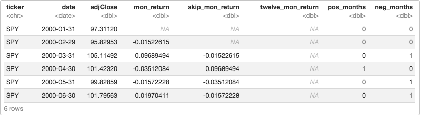
prices_monthly %>% mutate(mon_return = ((adjClose / lag(adjClose)) – 1), skip_mon_return = lag(mon_return)) %>% head()
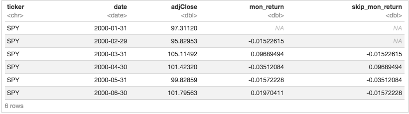
Have a quick peek at that data and notice how the skip_mon_return column is ignoring the previous month. For example, on March 31, 2001, we are not going to consider what happened from the end of February to the end of March, because there could be some weird stuff going on that’s isn’t going to last more than a few days. Instead, we’ll look back to what happened during February as our first data point.
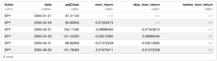
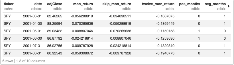
We also want to calculate the 12-months cumulative return, but we’ll lag that as well to with lag(adjClose) / lag(adjClose, 12) – 1).
prices_monthly %>% mutate(mon_return = ((adjClose / lag(adjClose)) – 1), skip_mon_return = lag(mon_return), twelve_mon_return = (lag(adjClose) / lag(adjClose, 12)) – 1) %>% head()
Let’s save this as an object called returns_tbl.
returns_tbl <-prices_monthly %>% mutate(mon_return = ((adjClose / lag(adjClose)) – 1), skip_mon_return = lag(mon_return), twelve_mon_return = (lag(adjClose) / lag(adjClose, 12)) – 1)
Now a basic momentum strategy might be to calculate if the twelve-month return exceeded some threshold, like 0, and if so, buy the asset for the following month.
We want to add a layer of logic that says, count the number of positive months over the preceding 12 months, and if equal to at least 8, encode a 1, else encode a 0.
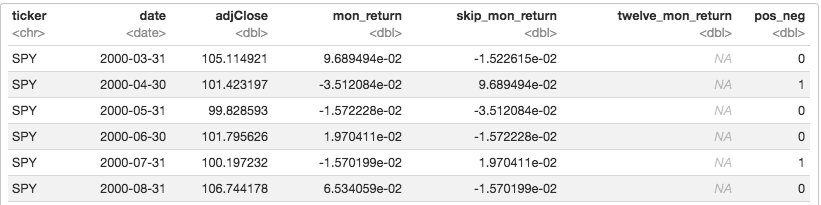
First, we label each month as positive or negative. If positive, label it 1, if negative label it 0. That will allow us to sum the positive months.
returns_tbl %>% slice(-1:-2) %>% mutate(pos_neg = case_when(skip_mon_return < 0 ~ 0, TRUE ~ 1))
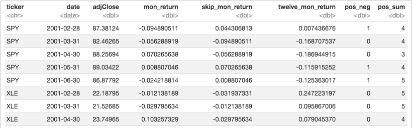
Next, we find the rolling sum of the pos_neg column.
returns_tbl %>% slice(-1:-2) %>% mutate(pos_neg = case_when(skip_mon_return < 0 ~ 0, TRUE ~ 1), pos_sum = rollsum(pos_neg, 12, fill = NA, align = “right”)) %>% slice(12:16)
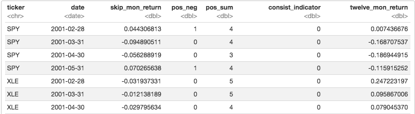
If the pos_sum is greater than or equal to 8, we label that period a 1. I’ll call that label the consist_indicator.
returns_tbl %>% slice(-1:-2) %>% mutate(pos_neg = case_when(skip_mon_return < 0 ~ 0, TRUE ~ 1), pos_sum = rollsum(pos_neg, 12, fill = NA, align = “right”), consist_indicator = case_when(pos_sum >= 8 ~ 1, TRUE ~ 0)) %>% select(ticker, date, skip_mon_return, pos_neg, pos_sum, consist_indicator, twelve_mon_return) %>% slice(12:16)
We now have an indicator for the consistency of the momentum. We can code up an algorithm that says if twelve_mon_return is positive and if consist_indicator is at least 8, then hold the asset for the following month, and code that time period as ‘quality’.
returns_tbl %>% slice(-1:-2) %>% mutate(pos_neg = case_when(skip_mon_return < 0 ~ 0, TRUE ~ 1), pos_sum = rollsum(pos_neg, 12, fill = NA, align = “right”), consist_indicator = case_when(pos_sum >= 8 ~ 1, TRUE ~ 0), strat_returns = if_else(lag(twelve_mon_return) > 0 & lag(consist_indicator) == 1, mon_return, 0), strat_label = if_else(lag(twelve_mon_return) > 0 & lag(consist_indicator) ==1, “quality”, “not_quality”)) %>% na.omit()
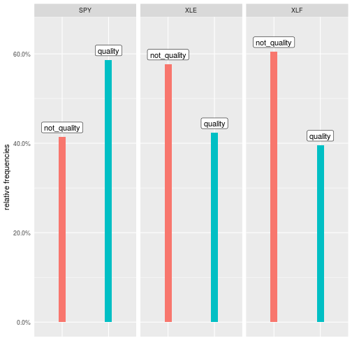
How frequently was each asset labeled ‘quality’?
returns_tbl %>% slice(-1:-2) %>% mutate(pos_neg = case_when(skip_mon_return < 0 ~ 0, TRUE ~ 1), pos_sum = rollsum(pos_neg, 12, fill = NA, align = “right”), consist_indicator = case_when(pos_sum >= 8 ~ 1, TRUE ~ 0), strat_returns = if_else(lag(twelve_mon_return) > 0 & lag(consist_indicator) == 1, mon_return, 0), strat_label = if_else(lag(twelve_mon_return) > 0 & lag(consist_indicator) ==1, “quality”, “not_quality”)) %>% na.omit() %>% count(strat_label) %>% mutate(prop = prop.table(n)) returns_tbl %>% slice(-1:-2) %>% mutate(pos_neg = case_when(skip_mon_return < 0 ~ 0, TRUE ~ 1), pos_sum = rollsum(pos_neg, 12, fill = NA, align = “right”), consist_indicator = case_when(pos_sum >= 8 ~ 1, TRUE ~ 0), strat_returns = if_else(lag(twelve_mon_return) > 0 & lag(consist_indicator) == 1, mon_return, 0), strat_label = if_else(lag(twelve_mon_return) > 0 & lag(consist_indicator) ==1, “quality”, “not_quality”)) %>% na.omit() %>% count(strat_label) %>% mutate(prop = prop.table(n)) %>% ggplot(aes(x = strat_label, y = prop, fill = strat_label)) + geom_col(width = .15) + scale_y_continuous(labels = scales::percent) + geom_label(aes(label = strat_label), vjust = -.4, fill = “white”) + ylab(“relative frequencies”) + xlab(“”) + expand_limits(y = .65) + theme(legend.position = “none”, axis.text.x = element_blank(), axis.ticks = element_blank()) + facet_wrap(~ticker)
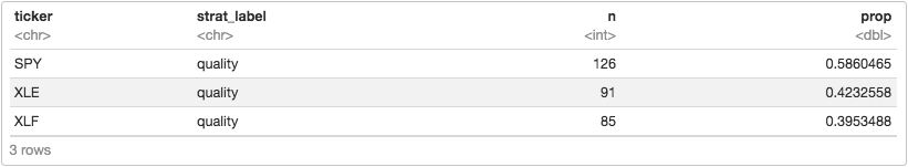
We also might want to sort these three by which had the highest proportion of quality periods.
returns_tbl %>% slice(-1:-2) %>% mutate(pos_neg = case_when(skip_mon_return < 0 ~ 0, TRUE ~ 1), pos_sum = rollsum(pos_neg, 12, fill = NA, align = “right”), consist_indicator = case_when(pos_sum >= 8 ~ 1, TRUE ~ 0), strat_returns = if_else(lag(twelve_mon_return) > 0 & lag(consist_indicator) == 1, mon_return, 0), strat_label = if_else(lag(twelve_mon_return) > 0 & lag(consist_indicator) ==1, “quality”, “not_quality”)) %>% na.omit() %>% count(strat_label) %>% mutate(prop = prop.table(n)) %>% filter(strat_label == “quality”) %>% arrange(desc(n))
This would be useful if we had 500 tickers and wanted to sort them into bins based on the number of quality periods. Perhaps next post we’ll go there, but for now let’s implement methodology two.
Alpha Architect “Frog in the Pan” Momentum
Recall the logic that we wish to encode: first, find the percentage of positive months, then find the percentage of negative months, subtract percentage of positive months from percentage negative months, multiply that result by the sign of the cumulative 12-months’ return. The result will be some number between -1 and 1.
Let’s go step-by-painstaking-step.
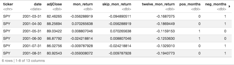
First, count the number of negative and positive months from the previous twelve months.
returns_tbl %>% mutate( pos_months = case_when(skip_mon_return > 0 ~ 1, TRUE ~ 0), neg_months = case_when(skip_mon_return < 0 ~ 1, TRUE ~ 0) ) %>% head()
Now we need the percentage of positive and negative months.
returns_tbl %>% slice(-1:-2) %>% mutate(pos_months = case_when(skip_mon_return > 0 ~ 1, TRUE ~ 0), neg_months = case_when(skip_mon_return < 0 ~ 1, TRUE ~ 0), pos_percent = rollsum(pos_months, 12, fill = 0, align = “right”)/12, neg_percent = rollsum(neg_months, 12, fill = 0, align = “right”)/12 ) %>% slice(-1:-12) %>% head()
And we want the difference between neg_percent and pos_percent, along with the sign() of the twelve_mon_return. Then we multiply those to get the information discreteness.
returns_tbl %>% slice(-1:-2) %>% mutate(pos_months = case_when(skip_mon_return > 0 ~ 1, TRUE ~ 0), neg_months = case_when(skip_mon_return < 0 ~ 1, TRUE ~ 0), pos_percent = rollsum(pos_months, 12, fill = 0, align = “right”)/12, neg_percent = rollsum(neg_months, 12, fill = 0, align = “right”)/12, perc_diff = neg_percent – pos_percent, pret = sign(twelve_mon_return), inf_discr = pret * perc_diff ) %>% slice(-1:-12) %>% head()
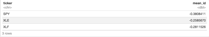
We have a measure of information discreteness for each 12-month period. Recall the minimum value for ID is -1, which indicates continuous information and high quality. Now we need a way to classify each stock as having a continuous or discrete ID score. We could find the mean ID score for each stock.
returns_tbl %>% slice(-1:-2) %>% mutate(pos_months = case_when(skip_mon_return > 0 ~ 1, TRUE ~ 0), neg_months = case_when(skip_mon_return < 0 ~ 1, TRUE ~ 0), pos_percent = rollsum(pos_months, 12, fill = 0, align = “right”)/12, neg_percent = rollsum(neg_months, 12, fill = 0, align = “right”)/12, perc_diff = neg_percent – pos_percent, pret = sign(twelve_mon_return), inf_discr = pret * perc_diff ) %>% slice(-1:-12) %>% summarise(mean_id = mean(inf_discr))
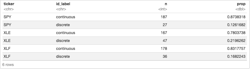
Or we could determine the number of 12-month periods that each had a negative score.
returns_tbl %>% slice(-1:-2) %>% mutate(pos_months = case_when(skip_mon_return > 0 ~ 1, TRUE ~ 0), neg_months = case_when(skip_mon_return < 0 ~ 1, TRUE ~ 0), pos_percent = rollsum(pos_months, 12, fill = 0, align = “right”)/12, neg_percent = rollsum(neg_months, 12, fill = 0, align = “right”)/12, perc_diff = neg_percent – pos_percent, pret = sign(twelve_mon_return), inf_discr = pret * perc_diff ) %>% slice(-1:-12) %>% mutate(id_label = case_when(inf_discr < 0 ~ “continuous”, TRUE ~ “discrete”)) %>% count(id_label) %>% mutate(prop = prop.table(n))
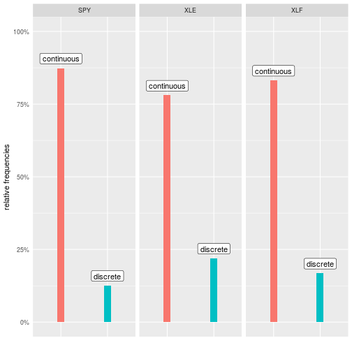
As before, let’s put this into a chart with ggplot.
returns_tbl %>% slice(-1:-2) %>% mutate(pos_months = case_when(skip_mon_return > 0 ~ 1, TRUE ~ 0), neg_months = case_when(skip_mon_return < 0 ~ 1, TRUE ~ 0), pos_percent = rollsum(pos_months, 12, fill = 0, align = “right”)/12, neg_percent = rollsum(neg_months, 12, fill = 0, align = “right”)/12, perc_diff = neg_percent – pos_percent, pret = sign(twelve_mon_return), inf_discr = pret * perc_diff ) %>% slice(-1:-12) %>% mutate(id_label = case_when(inf_discr < 0 ~ “continuous”, TRUE ~ “discrete”)) %>% count(id_label) %>% mutate(prop = prop.table(n)) %>% ggplot(aes(x = id_label, y = prop, fill = id_label)) + geom_col(width = .15) + scale_y_continuous(labels = scales::percent) + geom_label(aes(label = id_label), vjust = -.4, fill = “white”) + ylab(“relative frequencies”) + xlab(“”) + expand_limits(y = 1) + theme(legend.position = “none”, axis.text.x = element_blank(), axis.ticks = element_blank()) + facet_wrap(~ticker)
Conclusion
We wrote quite a bit of code to classify the quality of the momentum for three ETFs. Note that we could expand this to cover 10, 30, 100 or however many ETFs by adjusting the original ‘symbols’ object. The rest of the code would remain the same and we could scale this as large as we like.
For the curious, there’s a nice extension of the information discreteness calculation here via Newfound Research.
If you like this sort of thing check out my book, Reproducible Finance with R.
Not specific to finance but several of the ggplot tricks in this post came from this awesome Business Science University course.
Want to get into Momentum Investing? Have a look at this book Quantitative Momentum first.
Thanks for reading and happy coding!
- The views and opinions expressed herein are those of the author and do not necessarily reflect the views of Alpha Architect, its affiliates or its employees. Our full disclosures are available here. Definitions of common statistics used in our analysis are available here (towards the bottom).
- Join thousands of other readers and subscribe to our blog.
- This site provides NO information on our value ETFs or our momentum ETFs. Please refer to this site.
References
- Grinblatt, M., and T. Moskowitz. (2004). Predicting stock price movements from past returns: The role of consistency and tax-loss selling. Journal of Financial Economics 71:541–79
The post “Momentum, Quality, and R Code” appeared first on Alpha Architect.

