Predicting Equity Returns with Inflation

Key Points

Q2 2021 hedge fund letters, conferences and more

• Rather than predicting what will happen to inflation in the future—a particularly arduous and humbling task—we ask a simple question: What can past inflation dynamics tell us about the equity market’s future returns?
• We propose two new investment signals, which we label inflation cycles and surprises, and document that negative cycles and surprises predict higher equity returns in excess of the risk-free rate. We employ this predictability to design a new market-timing strategy: buy equities when inflation cycles and surprises are negative, and sell them otherwise.
• We show that the predictability of cycles and surprises varies across equity sectors. We exploit these differences in predictability to design a novel sector-rotating strategy.
• We highlight how inflation signals have worked consistently well across decades in addition to inflation and market regimes. Unlike commodities, tactical strategies based on inflation signals appear to perform well during both positive and negative market environments.

Michele Mazzoleni is the corresponding author.

Conversations in the investment industry have been dominated by predictions about the path of the inflation rate and its implications for capital markets. In this article, we aim to turn these conversations upside-down. We propose two new investment signals, which we call inflation cycles and inflation surprises. We find that negative cycles and surprises predict higher equity returns in excess of the risk-free rate, and we use this predictability to design a new market-timing strategy that buys equities when inflation cycles and surprises are negative, and sells them otherwise. We also show that the predictability of these signals varies across equity sectors and exploit these differences to design a novel sector-rotating strategy.

Why Inflation Dynamics Should Predict Risk Premia

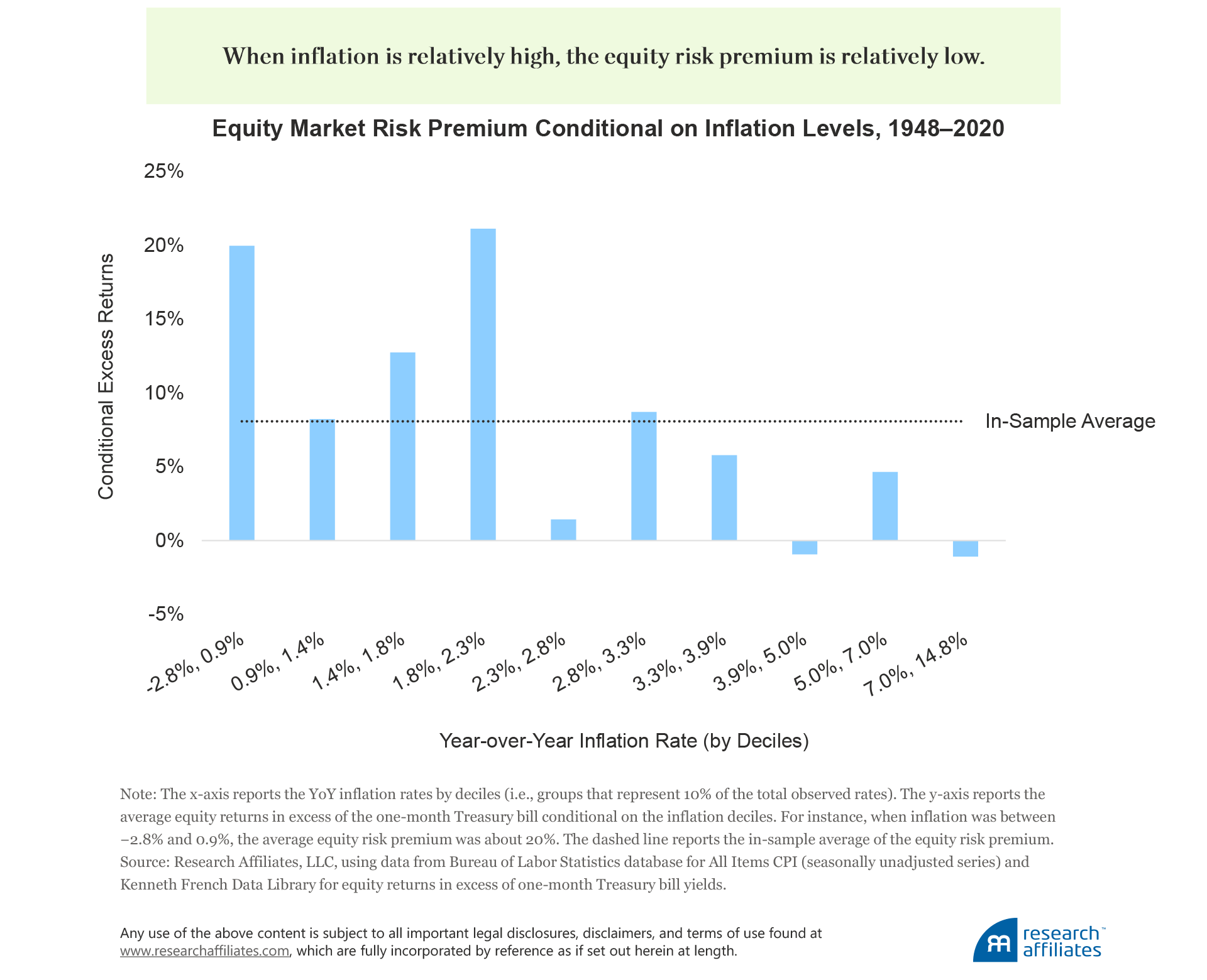
Multiple articles document that equity markets tend to underperform when inflation is relatively high.¹ To appreciate this relationship, we examine the average excess returns of the US stock market conditional on the contemporaneous year-over-year (YoY) inflation level for the period January 1948–December 2020. We find that when inflation is relatively high, the equity risk premium is relatively low, and is a statistically significant relationship. Unsurprisingly, today’s renewed inflation fears are dominating conversations in the investment industry. The determination of governments and central banks to provide support to their economies is leaving investors wondering whether prices may spiral as they did in the 1970s when inflation reached double digits.

The negative relationship between inflation rates and the equity risk premium may be unexpected to some because equities are a claim on real assets and, therefore, should provide a hedge against inflation. Fama (1981) offers an explanation for this evidence, noting that inflation may be a proxy for the business cycle and that periods of high inflation can coincide with periods of subdued real activity (i.e., stagflation). Related to this argument, Bekaert and Wang (2010) note that the discount rate channel likely plays a major role because risk premia increase during recessions (i.e., investors become more risk averse). We build and expand on these arguments by leveraging the Phillips Curve, a key concept in economics that classically relates inflation to unemployment.

In its modern version, the Phillips Curve is a reduced-form equation that connects the current inflation rate to inflation expectations and the business cycle. By approximating inflation expectations with an average of past inflation rates, we can generalize the Phillips Curve as follows:

Current Inflation Rate

Average of Past Inflation Rates + Output Gap

The Phillips Curve makes a simple point: Firms will react to changing expected costs of production. When costs are on the rise—for instance, when an economy is overheating—they trigger inflationary pressures as firms adjust their prices upward. The opposite should be true when aggregate production is relatively low. Accordingly, inflation dynamics should reflect a cyclical component related to the business cycle. More generally, the Phillips Curve is viewed as a key concept in guiding monetary policy. As explained by Federal Reserve Bank of New York President John Williams (2019): “The Phillips curve is the connective tissue between the Federal Reserve’s dual mandate goals of maximum employment and price stability.”

We leverage these insights from the economics literature and exploit them for a very different purpose—to predict asset prices. Our key analytical innovation is to interpret the difference between current and past inflation rates as a proxy for the state of the economy and employ it as a predictor of equities’ excess returns:

Investment Signal = Current Inflation Rate – Average of Past Inflation Rates

Output Gap

Underpinning our approach is the belief that the business cycle is related to investors’ risk appetite. Consistent with our view, Cooper and Priestley (2009) document that the output gap is a significant predictor of the equity market’s excess returns. If inflation dynamics are associated with real economic growth, they could also be a predictor of equities’ excess returns. In addition, metrics such as the potential level of output or employment are difficult to estimate and subject to a large degree of uncertainty. Therefore, inflation can provide an easily computable proxy of the business cycle.

From the Phillips Curve to Inflation Signals

To switch from an economic concept to an actionable investment strategy, we first need to “calibrate” the Phillips Curve and specify the Average of Past Inflation Rates term. For instance, should the average be computed with a long look-back window (i.e., a long “memory” series) or a short window (i.e., short memory)? We consider two solutions that effectively span the spectrum of options and result in the following two signals: 1) an inflation cycle and 2) an inflation surprise.

Let the inflation rate be defined as the year-over-year change in All Items CPI (seasonally unadjusted). We obtain an inflation cycle by subtracting from the current inflation rate an exponentially weighted moving average (EWMA) of past inflation rates, which resembles a “smooth” 10-year moving average. Hence,

Inflation Cycle = Current Inflation Rate – EWMA of Past Inflation Rates

We derive an inflation surprise as the difference between the current inflation rate and the previous month’s inflation rate:

Inflation Surprise = Current Inflation Rate – Previous Month Inflation Rate

Intuitively, an inflation cycle is indicative of longer-term trends in the growth rate of inflation—the long-memory series—whereas an inflation surprise reflects “news” about inflation dynamics.² We provide formal definitions of these signals in Appendix A.

We choose to focus on both cycle and surprise metrics based on the well-documented fall in inflation persistence over the last few decades.³ As noted by Williams (2019), this result implies that inflation surprises should no longer play a major role in driving inflation expectations and their effect should be of a transitory nature. Economists explain this phenomenon by arguing that inflation expectations have become “anchored” around the Federal Reserve’s target. In particular, the anchoring of inflation expectations suggests that in recent years moving averages with a relatively long memory should coincide with a more accurate approximation of these expectations, whereas in the earlier part of our sample, averages with a shorter memory should associate with greater accuracy.

Plotting the cycle and surprise series from January 1948 through December 2020, we find the correlation between the two series is 0.09, which suggests they capture different aspects of inflation dynamics. The average of the two series is indistinguishable from zero, which implies that the persistent component of inflation has been “purged” from the time series.⁴ We also note that inflation cycles are highly correlated with the original year-over-year inflation rate (correlation of 0.72). Indeed, periods of rising inflation tend to coincide with periods of relatively high inflation (on average 5.4%), and times of falling inflation tend to coincide with times of relatively low inflation (on average 2.1%).

Cooper and Priestly (2009) document that positive output gaps associate with future lower equity excess returns. Consistent with their work, we expect that positive inflation signals should also associate with lower risk premia. In addition, because of the changing nature of inflation dynamics, we expect inflation surprises to display stronger predictive power in the earlier part of our sample, whereas inflation cycles should perform better over the last three decades.

Timing the US Equity Market with Inflation Signals

We convert inflation cycles and surprises to investment signals by taking their sign: +1 if the cycle or surprise is positive (rising inflation), and –1 if it’s negative (falling inflation). We call these and for cycles and surprises, respectively. Equipped with these two signals we simulate the returns of two self-financed portfolios that trade the US equity market. If a signal was negative during the previous month (falling inflation), our strategy buys equities and finances the position with the one-month Treasury bill.⁵ If the signal was positive (rising inflation), the strategy sells the market and invests in the risk-free rate. The goal of the strategy is to profit by going long equities when inflation has been falling and by shorting them otherwise. The equity data start in January 1948 and are from the Kenneth French Data Library, while the inflation data are from the Bureau of Labor Statistics. We employ seasonally unadjusted All Item CPI, which is an unrevised series, and we lag it by a full calendar month to avoid look-ahead biases (we provide more details in Appendix B).

To test the strategy, we create portfolios based on the inflation-cycle and inflation-surprise signals, which we label Cycles Portfolio and Surprises Portfolio, and also create a portfolio that is their average (Average Portfolio). As points of reference, we compare the returns of these portfolios with the excess returns of a long position in the equity market as well as a time-series momentum portfolio (TSMOM), which goes long, neutral, or short based on the sign of trailing 1- and 12-month excess returns.6 The alpha of the portfolios are calculated with respect to a simple long position in the equity market, and we report their statistical significance (t-Statistic). We summarize our evidence in the following table:

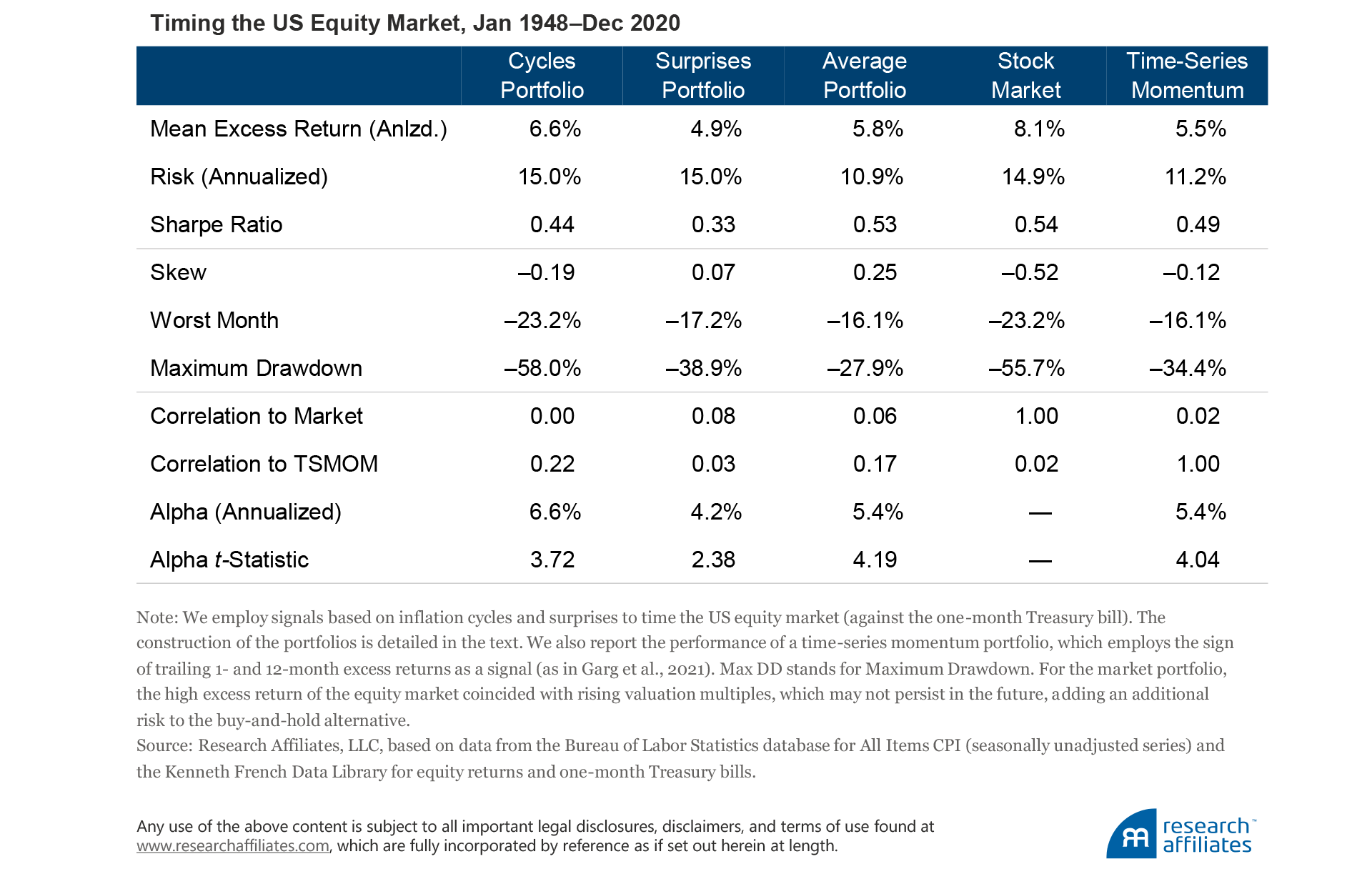
Our evidence suggests that inflation signals are indeed significant predictors of equities’ excess returns. Both signals translate into statistically and economically meaningful alpha; the cycles signal delivered the strongest outperformance. In particular, the premium harvested from combining the inflation signals is comparable to the one earned by the well-documented time-series momentum portfolio, while the two strategies themselves are not highly correlated (0.09).

“Inflation signals are indeed significant predictors of equities’ excess returns. Both signals (cycles and surprises) translate into statistically and economically meaningful alpha.”

We highlight how the inflation signals capture different dynamics of the equity market. The correlation between the two tactical portfolios stands at only 0.02, so the Average Portfolio delivers higher risk-adjusted excess returns. In addition, the “lives” of the cycle and surprise signals are quite different. By construction, inflation cycles tend to persist over time, so the decay of the signal is relatively slow. In contrast, the decay of inflation surprises is much faster, because the signal displays little persistence, even over a monthly horizon.

Timing US Equity Sectors with Inflation Signals

Inspired by our market-level results, we move to a finer level of analysis by investing in individual equity sectors. Our prior is that different sectors should display different sensitivities (betas) to inflation signals and that these differences should translate into different performances across inflation regimes. Whereas all sectors may struggle following rising inflation rates, as Neville et al. (2021) document, some sectors may struggle more than others. The evidence shows exactly that.

We summarize the forecasting power of the cycle and surprise metrics across 10 sectors as well as the aggregate market and across two periods (before and after 1990).⁷ For each sector j and the market, we run individual regressions of excess returns on the signals of cycles () or surprises (). We then report the t-statistic associated with these predictive relationships. As expected, both inflation signals are negatively associated with future excess returns across all sectors, meaning rising inflation corresponds to falling returns.

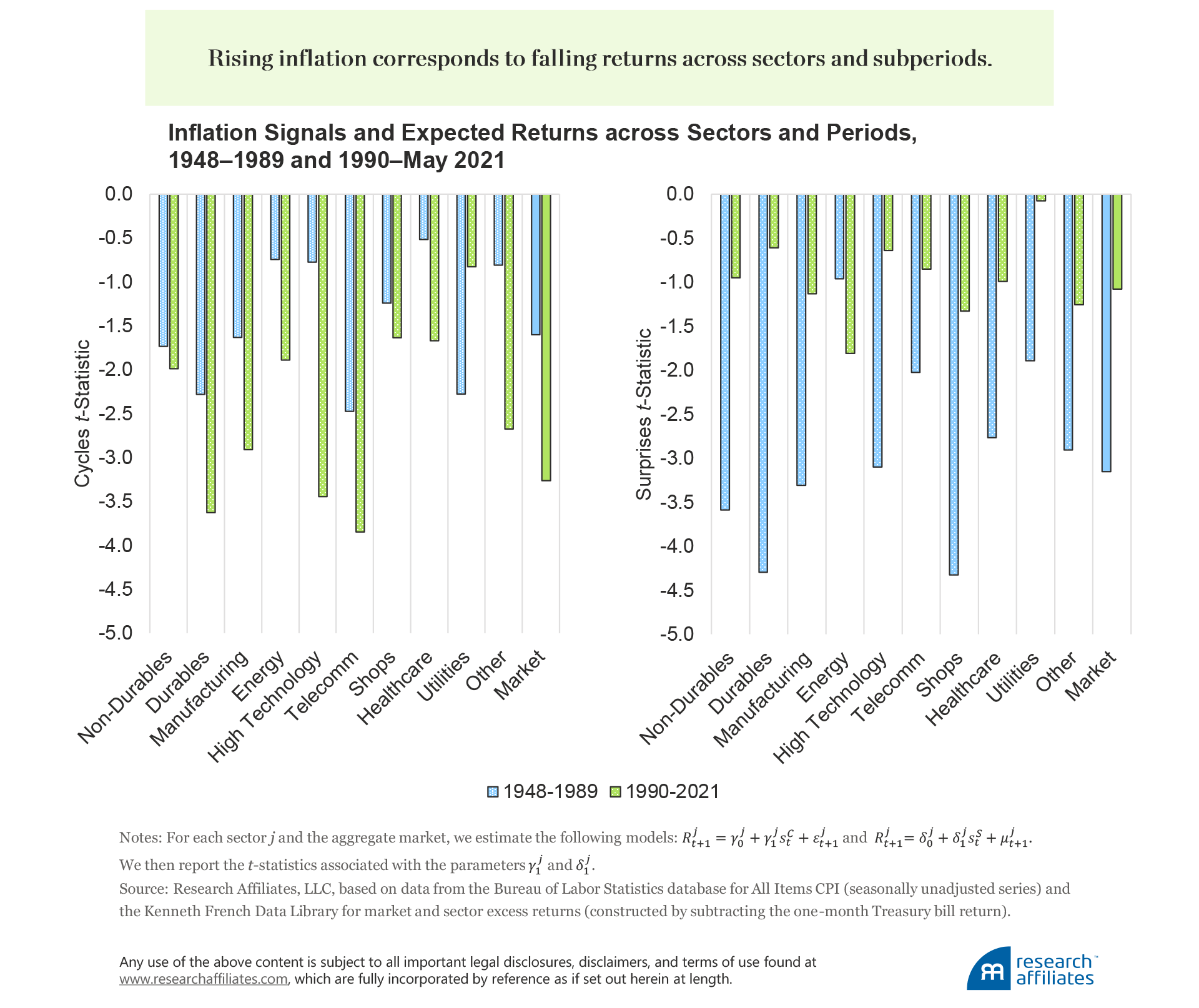
As hypothesized in the previous section, the predictability of cycles and surprises does indeed vary across decades. In recent years, inflation cycles have become a stronger predictor, whereas surprises have lost the lion’s share of their predictive power. These patterns are present across the majority of the sectors. We infer that, for the most recent decades, inflation expectations can be better approximated by employing moving averages with longer look-back windows; the opposite is true for the period of the 1970s and 1980s.

We also highlight some intuitive differences across sectors: the predictive power tends to be the strongest for durables, which includes the automobile sector, and least successful for the energy-related sectors: energy and utilities. In general, these patterns can be explained via a complementarity channel. Inflation measures the changing price of different goods and services produced by different industries. Some of them are complementary goods, such as gasoline and cars, for which a price increase in one good leads to a decrease in the demand of the other good (an effect known as negative cross-elasticity of demand). We argue that the most predictable industries display the highest degree of complementarity to energy goods and services, and therefore struggle the most during periods of rising inflation. Yet, exceptions may occur, as in the case of tech firms, for which the duration channel is the most likely driver of sensitivity to inflation.

Read the full article here by Jim Masturzo, Michele Mazzoleni – Research Affiliates