
Over the last three years, Euclidean has engaged in an intense research and development effort to assess whether the great advances in machine learning achieved in the past decade can improve our systematic, long-term investing processes. This article is the first in a several-part series that describes what we have learned from this research process.
Q1 2021 hedge fund letters, conferences and more
We were motivated by the fact that newly developed deep learning technologies had shown great progress in three areas that seemed beneficial to financial modeling: learning sequences, working with unstructured (financial) data, and learning textual data. In the end, we found that the first two greatly improved what we could achieve with our long-term investment models. The last (learning textual data) is still an intense and exciting active research area at Euclidean. This note is the first part of our explaining the journey that brought us to our findings.
Background
When evaluating companies as potential investments, we can look at their pasts. We can compare them to other companies and consider how they performed as investments. But, ultimately, how companies evolve and how their share prices perform will be driven by future developments that we cannot observe in advance.
So, in this sense, our reviewing data and looking at comparable situations from the past is meant to help us anticipate the future. We seek to establish base rates for how companies with certain sets of characteristics, when offered at certain prices, typically have performed. We then invest in companies with favorable comparables, believing that doing so puts the long-term odds on our side.
However, this is all just a proxy for what ultimately matters, which is simply whether a company’s future earnings develop more or less favorably than the market expects. Yes, some companies trade on revenues or developments other than earnings, but, over time, companies’ long-term market values generally have moved toward what their earnings dictated [1]. Thus, in line with common sense, it seems that, the better you can forecast earnings and invest in companies that are priced low in relation to those future earnings, the greater your opportunity for future returns.
To test the validity of our intuition, we ran simulations with a clairvoyant model that accesses future fundamentals, such as sales, operating earnings (earnings before interest and taxes; EBIT), book value, free cash flow, etc. Obviously, we can’t know the future, but we can use historical data to simulate how well we’d perform if we did know the future.
With such historical data, we can create factors, such as the future EBIT divided by the current enterprise value (EV). In the figure below, we plot the annualized return of these factors from 2000 to 2019 for different clairvoyance periods [2]. In line with our intuition, the further we move into the future, the better the portfolio performance becomes. Future operating income divided by EV proves to be the best performing factor, while free cash flow divided by EV comes in as a close second.
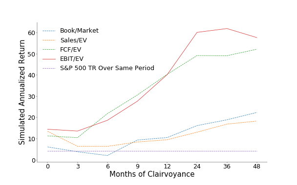
Annualized return for different clairvoyance periods
So, if we could have known the fundamentals 12 months into the future, we could have achieved an annualized return (again, hypothetically) of 40%. Consider that in comparison to a 14% annualized return for the traditional model, which uses current EBIT. This, therefore, motivates us to predict future fundamentals. We ask ourselves if we can, by forecasting future fundamentals, close the performance gap between using current and using future fundamentals and, thus, realize some of those gains.
Why Deep Learning?
Ever-increasing data and advances in computing power launched innovations in deep learning, which have led to significant progress over the last decade. Now, more than ever, machine learning models can uncover complex and fruitful patterns that lay hidden in highly complex environments. Deep learning is behind the much talked about achievements of self-driving cars, image recognition technology that performs better than humans, impressive language translation, and voice recognition.

Applications of machine learning in computer vision, language translation, and games like Go. Source – Nvidia, Google Translate, Deepmind.
Deep learning techniques are aptly suited for financial modeling. Deep Neural Networks (DNNs) can identify complex and non-linear relationships that we may (or may not) be able to identify via feature engineering. Additionally, economic data is sequential in nature. Tools from natural language processing research allow us to understand financial sequences much better and are discussed in detail in this post. These same language tools can be used to exploit a vast amount of unstructured textual data, such as the U.S. Securities and Exchange Commission (SEC) filings and call transcripts.
Hence, following the clairvoyant study, we set our objective to forecast EBIT using deep learning. We chose EBIT as it is less lumpy than cashflow, but the same approach can be applied to cashflow, as well. In practice, we forecast multiple fundamentals because it helped avoid overfitting. We used a forecast period of 12 months, as it provided the best trade-off between the accuracy of the forecasting model and the portfolio performance. Obviously, the further into the future we had to make a prediction, the less accurate it was. We will discuss this in detail later. The figure below shows some examples of the forecasts made by the deep learning model.
Deep learning forecasts and uncertainty bounds of earnings (80% credible intervals); model was trained from Jan 1, 1970 to Jan 1, 2000.
The Data
Before discussing the deep learning models, it is important to understand the data behind them. We sourced the data from 1970 to 2019. Because reported information arrives intermittently throughout a financial period, we discretized the raw data into a monthly time step. We were interested in long term predictions, and, to smooth out seasonality every month, we fed a time series of inputs with a one-year gap between the time steps and predicted the earnings one year into the future from the last time step. For example, one trajectory in our dataset consisted of data for a given company from (Jan 2000, Jan 2001, …, Jan 2004), which was used to forecast earnings for Jan 2005. For the same company, we also had another trajectory consisting of data from (Feb 2000, Feb 2001, …, Feb 2004), which was used to forecast earnings for Feb 2005.
Sample time series data structure
We used three classes of time series data: fundamental features, momentum features, and auxiliary features. Fundamental features included the data from a company’s financial statements. Momentum features included one-, three-, six-, and nine-month relative momentum (change in stock price) for all stocks in the universe at the given time step. Auxiliary features included any additional information we thought was important, such as short interest, industry sector, company size classification, etc. In total, we used about 80 input features.
Deep Learning Model
Our goal was to forecast future fundamentals, specifically EBIT. But how does the model go about doing that? Let’s say there is a 12-year-old restaurant chain operator with $200 million in revenue and a market capitalization of $800 million. What we hope is that our model has seen patterns of companies similar to this one during training and has learned to identify them. Companies that are similar in terms of size, growth trajectory, business characteristics, financial statements, etc., can help determine the forward trajectory of this restaurant chain operator. The more examples the model sees during training, the better it gets at identifying such patterns—hopefully making better forecasts. In theory, this is what a good bottom-up investment analyst does. The advantage of using machine learning is that we can look at a large number of dimensions, learn the complex relationships in the data, and examine many more historical examples.
We used DNNs to predict future fundamental features given a time series of inputs. One advantage of deep learning is that it can handle raw, unstructured data, so intense feature engineering is not required. We also employed Recurrent Neural Networks (RNNs), commonly used in natural language processing, which helped exploit the temporal nature of the financial data.
For example, consider this sentence, “The cat ate all the food, as it was hungry.” An RNN model processes data sequentially and can understand the relationship between two words, not just by their meaning, but also by their position. The model knows “it” refers to the word “cat” rather than to “food.”
A time step in a financial time series can be thought of as a word in a sentence. Financial metrics across time, just like words, are not independent of each other, but are temporally related. How the business changed from one year to the next over the last five years is important when forecasting next year’s performance. Hence, we looked at the interaction of input features across time, which a simpler model would fail to do. In the figure below, the green cells represent neural network units. Each cell contains information about previous cells, as indicated by the red arrows; this allows the network to learn temporally important relationships.
RNNs process data sequentially, learning temporal relationships in the sequence.
We chose the input sequence to consist of a five-year time series of data, with an annual time step. We set the output to be EBIT one year from the last time step [3]. EBIT was, therefore, required to calculate the factor driving the investment model. Although we cared about EBIT, we forecast all the fundamentals using the same neural network. This is known as Multitask Learning, which helps control overfitting. To ensure that the model was more sensitive to the EBIT’s accuracy, we upweighted its effect in the loss function the model was attempting to minimize.
Each green cell in the previous figure is a neural network that uses input from one year to output fundamentals at the next time step; EBIT is up-weighted in the loss function
With any forecasting model, the objective is to maximize the model’s accuracy. In training neural networks, this is achieved by iteratively minimizing the error between the target and predicted values via the aforementioned loss function.
To simulate how a machine learning model will perform in real time, we tested its performance on an unseen or out-of-sample dataset. In this experiment, we divided the timeline into in-sample and out-of-sample periods. We trained the model using the in-sample period of 1970 to 1999, and, thus, the out-of-sample (test) period stretched from 2000 to 2019.
You may wonder if a model that has only learned data from 1970–1999 is qualified to make a prediction for a company in 2019, since the economic and market environments may have changed significantly. As business characteristics and industries do change over time, this is a valid question. In practice, we train our model iteratively. For every year for which we forecast the EBIT, we train a separate model with the prior 30 years of historical data. This ensures that the model always receives the most recent information. However, in the experiments described in this article, we restricted the training period to 1970–1999 and the test period to 2000–2019 for simplicity.
Uncertainty and Risk
Forecast models are primarily judged by their accuracy. However, as important as accuracy is, it does not offer the complete picture. Imagine the computer vision system in a self-driving car on a rainy night. It may conclude that the road ahead is clear, but don’t we also want to know how confident the system is about its assessment? The same is true in finance; our models should be able to tell, not only the forecasts, but also how confident they are in the forecasts they are making. We can then use that information to aid our decision-making.
If a model is uncertain about its prediction, we treat it as riskier and adjust the forecast accordingly. Say we have two similarly sized companies—a cyclical semiconductor company, with highly volatile earnings, and a stable consumer packaged goods (CPG) company. Assume further that both companies have the same enterprise value of $1B, and the model forecasts $100M in operating income, resulting in a future earnings yield (EY) of 10%. Even though the future EY is the same, we may feel more confident in one forecast over the other because of how the businesses and their respective industries operate.
So, concretely, we want the model to output uncertainty estimates for each prediction, which we will then use to adjust the forecast. There are multiple sources of uncertainty (or noise) in this forecasting process. We have focused on two types of noise—the first being the noise within the model. No model is perfect. This type of noise tries to capture the limitations of the model and/or the fact that the data might not include all the necessary information for making the prediction.
Second is the noise within the data itself. This is especially critical in financial and economic data. Much financial data depends on human behavior, which is inherently noisy, as opposed to a physics experiment. Two companies, which are very similar with respect to their historical financials, might still have wildly different business outcomes because of exogenous factors (e.g., one company loses their largest customer). Additionally, the noise level during a moment of crisis, such as the 2008–2009 Global Financial Crisis, is very different from that during a relatively stable period, and it depends on the underlying data.
In our deep learning model, we estimated both types of noise. For the model noise, we built multiple models, calculated their variance, and combined the results to obtain more robust predictions. For the data noise, we used the same deep learning model to output data-dependent variance. We included this variance in the objective function along with accuracy. The objective function then attempted to maximize accuracy while minimizing variance. The model was penalized if it returned an accurate prediction at a low confidence level (high variance), and the same was true for an overconfident model with bad predictions. Training a model is a balancing act between these two objectives.
The output layer is split into mean and variance output nodes. Sharing network weights enables variance to be data dependent.
In this way, we retrieved the uncertainty estimate in the form of total variance, which is a combination of model noise and data noise. We then scaled the prediction in inverse proportion to the noise estimate. This was akin to saying we were not very confident that company XYZ would make $100M, but it might have a better shot at making $50M. We then created the ranking factor using the enterprise value to make investing decisions.
In the next post, we will discuss in detail how these factors were created, along with the portfolio simulation process. Finally, we will look at the results of these experiments and the value they provide to a systematic, long-term investing process like ours.
Footnotes:
[1] Price Earnings Ratios as a Predictor of 20-Year Returns (Shiller Data) and Do Stock Prices Move Too Much to be Justified by Subsequent Changes in Dividends? (Shiller).
[2] The clairvoyance period refers to how far into the future we were looking. A 12-month clairvoyance period meant we had access to fundamentals 12 months into the future.
[3] We selected EBIT as the output because the clairvoyance study showed that the EBIT/EV factor outperformed all other factors.
Article by Lakshay Chauhan and John Alberg, Euclidean

