
Imagine approaching a friend that you think is very wealthy and asking her to borrow ten thousand dollars for just one night. To entice her, you offer as collateral the title to your 2019 Lexus parked in her driveway along with an interest rate that is 5% above that which she is earning in the bank. Shockingly, your friend says she can’t. Given the risk-free nature of the transaction and excellent one-day profit, we can assume that our friend may not be as wealthy as we thought.
Q2 hedge fund letters, conference, scoops etc
On Monday, September 16th, 2019, a similar situation occurred in the overnight repurchase agreement (repo) funding market. On that day, banks were unwilling or unable to lend on a collateralized basis, even with the promise of large risk-free profits. This behavior reveals something very important about the banking system and points to the end of market stimulus that has been around for the past decade.
The Plumbing of the Banking System and Financial Markets
Interbank borrowing is the engine that allows the financial system to run smoothly. Banks routinely borrow and lend to each other on an overnight basis to ensure that all banks have ample funds to meet daily cash flow needs and that banks with excess funds can earn interest on them. Literally, years go by with no problems in the interbank markets and not a mention in the media.
Before proceeding, what follows is a definition of the funding instruments used in the interbank markets.
- Fed Funds are uncollateralized interbank loans that are almost exclusively done on an overnight basis. Except for a few exceptions, only banks can trade Fed Funds.
- Repo (repurchase agreements) are collateralized loans. These transactions occur between banks but often involve other non-bank financial institutions such as insurance companies. Repo can be negotiated on an overnight and longer-term basis. General collateral, or “GC,” is a term used to describe Treasury, agency, and mortgage collateral that backs certain repo loans. In a GC repo, the particular securities backing the loan are not determined until after the transaction is agreed upon by the counterparties. The securities delivered must meet certain pre-defined criteria.
On September 16th, overnight GC repo traded as high as 8%, almost 6% higher than the Fed Funds rate, which theoretically should keep repo and other money market rates closely tied to it. The billion-dollar question is, “Why did a firm willing to pay a hefty premium, with risk-free collateral, struggle to borrow money”? Before the 16th, a premium of 25 to 50 basis points versus Fed Funds would have enticed a mob of financial institutions to lend money via the repo markets. On the 16th, many multiples of that premium were not enticing enough.
Most likely, there was an unexpected cash crunch that left banks and/or financial institutions underfunded. The media has talked up the corporate tax date and a large Treasury bond settlement date as potential reasons. We are not convinced by either excuse as they were easily forecastable weeks in advance.
Regardless of what caused the liquidity crunch, we do know, that in aggregate, banks did not have the capacity to lend money. Given the capacity, they would have done so in a New York minute and at much lower rates.
To highlight the enormity of the aberration, consider the following:
- Since 2006, the average daily difference between the overnight GC repo rate and the Fed Funds effective rate was .025%.
- Three standard deviations or 99.5% of the observances should have a spread of .56% or less.
- 8% is a bewildering 42 standard deviations from the average, or simply impossible assuming a traditional bell curve.
What was revealed on the 16th?
The U.S. and global banking systems revolve around fractional reserve banking. That means banks need only hold a fraction of the cash deposits that they hold in reserve accounts at the Fed. For example, if a bank has $1,000 in deposits (a liability to the bank), they may lend $900 of those funds and retain only 10% in reserves. This is meant to ensure they have enough funding on hand to make payments during the day and also as a buffer against unanticipated liquidity needs. Before 2008, banks held only just as many reserves as were required by the Fed. Holding anything more than the required minimum was a drag on earnings, as excess reserves were unremunerated at the time.
Quantitative Easing (QE) and the need for the Fed to pay interest on newly formed excess reserves changed that. When the Fed conducted QE, they bought U.S. Treasury, agency, and mortgage-backed securities and credited the selling bank’s reserve account. The purpose of QE1 was to ensure that the banking system was sufficiently liquid and equipped to deal with the ramifications of the ongoing financial crisis. Round one of QE was logical given the growing list of bank/financial institution failures. However, additional rounds of QE appear to have had a different motive and influence as banks were highly liquid after QE1 and had shored up their capital as well. That is a story for another day.
The graph below shows how “excess” reserves were close to zero before 2008 and soared by over $2.5 trillion after the three rounds of QE. Before QE, “excess” reserves were tiny, measured in the hundreds of millions. The amount is so small it is not visible on the graph below. The reserves produced by multiple rounds of quantitative easing may have been truly excess, meaning above required reserves, on day one of QE. However, on day two and beyond that is not necessarily true for any particular bank or the system as a whole, as we are about to explain.
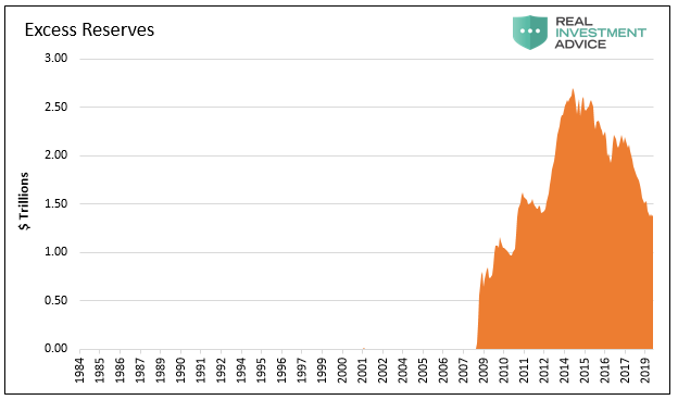
Data courtesy: St. Louis Federal Reserve
The Fed, having pushed an enormous amount of reserves on the banks, created a potential problem. The Fed feared that once the smoke cleared from the financial crisis, banks would revert to their pre-crisis practice of keeping only the minimum amount of reserves required. This would leave them an unprecedented surplus of excess funds to buy financial assets and/or create loans which would vastly increase the money supply with inflationary consequences. To combat this problem, they incentivized the banks to keep the reserves locked down by paying them a rate of interest on the reserves that were higher than the Fed funds rates and other prevailing money market rates. This rate is called the IOER or the interest on excess reserves.
The Fed assumed banks would hold excess reserves because they could make risk free profits at no cost. This largely worked, but some reserves were leveraged by the banks and flowed into the financial markets. This was a big factor in driving stock prices higher, credit spreads tighter, and bond yields lower. This form of inflation the Fed seemed to desire as evidenced from their many speeches talking about generating household net worth.
From the banks’ perspective, the excess reserves supplied by the Fed during QE were preferential to traditional uses of excess reserves. Historically, excess bank reserves were invested in the Treasury market or lent on to other banks in the Fed Funds market. Purchasing Treasury securities had no credit risk, but banks are required to mark their Treasury holdings to market and therefore produce unexpected gains and losses. Lending reserves in the interbank market also incurred counterparty risk, as there was always the chance the borrowing bank would be unable to repay the loan, especially in the immediate post-crisis period. Additionally, as QE had produced trillions in excess reserves, there was not much demand from other banks. Therefore, the banks preferred use of excess reserves was leaving them on deposit with the Fed to earn IOER. This resulted in no counterparty risk and no mark to market risk.
Beginning in 2018, the Fed began reducing their balance sheet via QT and the amount of excess reserves held by banks began to decline appreciably.
Solving Our Mystery
It is nearly impossible for the public to figure out how much in excess reserves the banking system is truly carrying. Indeed, even the Fed seems uncertain. It is common knowledge that they have been declining, and over the last six months, clues emerged that the amount of “truly excess reserves,” meaning the amount banks could do without, was possibly approaching zero.
Clue one came on March 20th, 2019 when the Fed said QT would end in October 2019. Then, on July 31st, 2019, as small problems occurred in the funding markets, the Fed abruptly announced that they would halt the balance sheet reduction in August, two months earlier than originally planned. The QT effort, despite assurances from Bernanke, Yellen, and Powell that it would be uneventful, ended 22 months after it began. The Fed’s balance sheet declined only $800 billion as a result of QT, less than a quarter of what the Fed added to their balance sheet during QE.
Clue two was the declining spread between the IOER rate and the effective Fed Funds rate as the level of excess reserves was declining, as seen in the chart below. The spread between IOER and the Fed Funds rate was narrowing because the Fed was having trouble maintaining the Fed Funds rate within the targeted range. In March 2019, the spread became negative, which was counter to the Fed’s objectives. Not surprisingly, this is when the Fed first announced that QT would end.
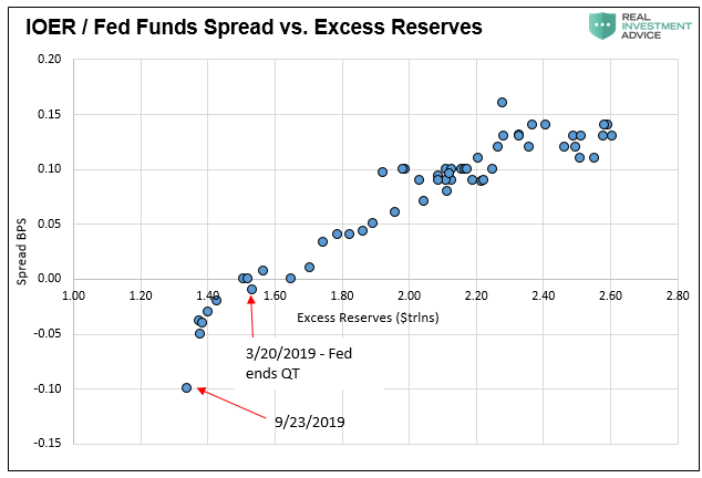
Data courtesy: St. Louis Federal Reserve
The third and final clue emerged on September 16, 2019, when overnight repo traded at 7%-8%. If banks truly had excess reserves, they would have lent some of that excess into the repo market and rates would never have gotten close to 7-8%. It seems logical that banks would have been happy to lend on a collateralized basis at 3%, much less 7-8%, when their alternative, leaving excess reserves to the Fed, would have earned them 2.25%.
Further confirmation that something was amiss occurred on September 17th, 2019, when the Fed Funds effective rate was above the upper end of the Fed’s target range of 2-2.25% at the time. This marked the first time the Fed Funds rate traded above its target since 2008.
On September 17th, the Fed entered the repo markets with a $53 billion overnight repo operation, whereby banks could pledge Treasury collateral to the Fed and receive cash. The temporary liquidity injection worked and brought repo rates back to normal. The following day the Fed pumped $75 billion into the markets. These were the first repo transactions executed by the Fed since the Financial Crisis, as shown below.
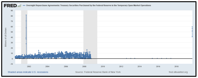
These liquidity operations will likely continue as long as there is demand from banks. The Fed will also conduct longer-term repo operations to reduce the amount of daily liquidity they provide.
The Fed can continue to resort to the pre-QE era tactics and use temporary daily operations to help target overnight borrowing rates. They can also reduce the reserve requirements which would, at least for some time, provide the system with excess reserves. Lastly, they can permanently add reserves with QE. Recent rhetoric from Fed Chairman Powell and New York Fed President Williams suggests a resumption of QE in some form may be closer than we think.
Why should we care?
The QE-related excess reserves were used to invest in financial assets. While the investments were probably high-grade liquid assets, they essentially crowded out investors, pushing them into slightly riskier assets. This domino effect helped lift all asset prices from the most risk-free and liquid to those that are risky and illiquid. Keep in mind the Fed removed about $3.6 trillion of Treasury and mortgage securities from the market which had a similar effect.
The bottom line is that the role excess reserves played in stimulating the markets over the last decade is gone. There are many other factors driving asset prices higher such as passive investing, stock buybacks, and a broad-based, euphoric investment atmosphere, all of which are byproducts of extraordinary monetary policies. The new modus operandi is not necessarily a cause for concern, but it does present a new demand curve for the markets that is different from what we have become accustomed to.
Summary
Short-term funding is never sexy and rarely if ever, the most exciting part of the capital markets. A brief recollection of 2008 serves as a reminder that, when it is exciting, it is usually a harbinger of volatility and disruption.
In a Washington Post article from 2010, Bernanke stated, “We have made all necessary preparations, and we are confident that we have the tools to unwind these policies at the appropriate time.”
Much more recently, Jay Powell stated, “We’ve been operating in this regime for a full decade. It’s designed specifically so that we do not expect to be conducting frequent open market operations to keep fed fund [sic] rates in the target range.”
Today, a decade after the financial crisis, we see that Bernanke and Powell have little appreciation for the inner-workings of the financial system.
In the Wisdom of Peter Fisher, an RIA Pro article released in July, we discussed the insight of Peter Fisher, a former Treasury, and Federal Reserve official. Unlike most other Fed members and politicians, he discussed how hard getting back to normal will be. As we are learning, it turns out that Fisher’s wisdom from 2017 was visionary.
“As Fisher stated in his remarks, “The challenge of normalizing policy will be to undo bad habits that have developed in how monetary policy is explained and understood.” He continues, “…the Fed will have to walk back from their early assurances that the “exit would be easy.”
Prophetic indeed.
Article by Michael Lebowitz, CFA and Jack Scott CFA – Real Investment Advise

